
Relational Database and MySQL
DATABASE MANAGEMENT SYSTEM
1. Database
A Database is an organized collection of data, it can be visualized as a container of information.
2. Database Management System
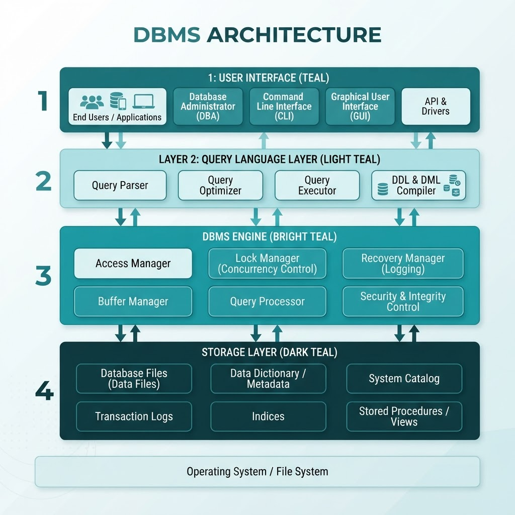
DBMS is a software package with computer programs that control the creation, maintenance, and use of a database. A database is a collection of data and DBMS allows different user application programs to concurrently access the same database.
Examples of DBMS: Oracle, MySQL, FoxPro, IBM DB2, Microsoft SQL Server, OpenOffice.org Base, and Microsoft Access.
3. Organization of Data
Data can be organized in two ways:
- Flat File: Data is stored in a single table. This is usually suitable for less amount of data.
- Relational: Data is stored in multiple tables which are linked by a common field. This is suitable for medium to large amount of data.
4. Database Servers
These are dedicated computer systems that hold the databases and run only the DBMS and related software. Databases are available on database servers and are usually accessed through a command line or Graphic User Interface tools (called Frontend).
5. Limitations and Disadvantages
- Data redundancy (Duplication of data)
- Data inconsistency
- Unreliable data
- Unstandardized data
- Insecure data
- Incorrect data
6. Advantages of Database
6.1 Reduces Data Redundancy
Database reduces data redundancy. Database reduces Duplication of data, in fact, there is no chance to encounter duplicate data in a database.
6.2 Reduce Data Inconsistency
Multiple mismatching copies of same data is known as data inconsistency.
6.3 Sharing of Data
The users of the database can share the data among themselves.
6.4 Data Integrity
Data integrity means that the data in the database is accurate and consistent.
6.5 Data Security
Database provides data security as only authorized users are allowed to access the database and their identities are authenticated by using a username and password.
6.6 Privacy
Only authorized users can access a database according to the database privacy constraints.
6.7 Backup and Recovery
DBMS automatically takes care of backup and recovery. In case of a crash or system failure, it gets restored to its previous condition.
7. Features of Database
- The database has one or more tables.
- Each table has information about one type of item.
- Every table in a database has a key field that makes sure that there are unique values throughout the database.
8. Keys in a Database
8.1 Primary Key
A primary key is a unique value that identifies a row in a table. Primary Key helps the database to quickly search for a record. Cannot contain null values.
8.2 Composite Primary Key
When a primary key constraint is applied on one or more columns then it is known as Composite Primary Key.
8.3 Foreign Key
The foreign key identifies a column or set of columns in one (referencing) table that refers to a column or set of columns in another (referenced) table.
9. Table
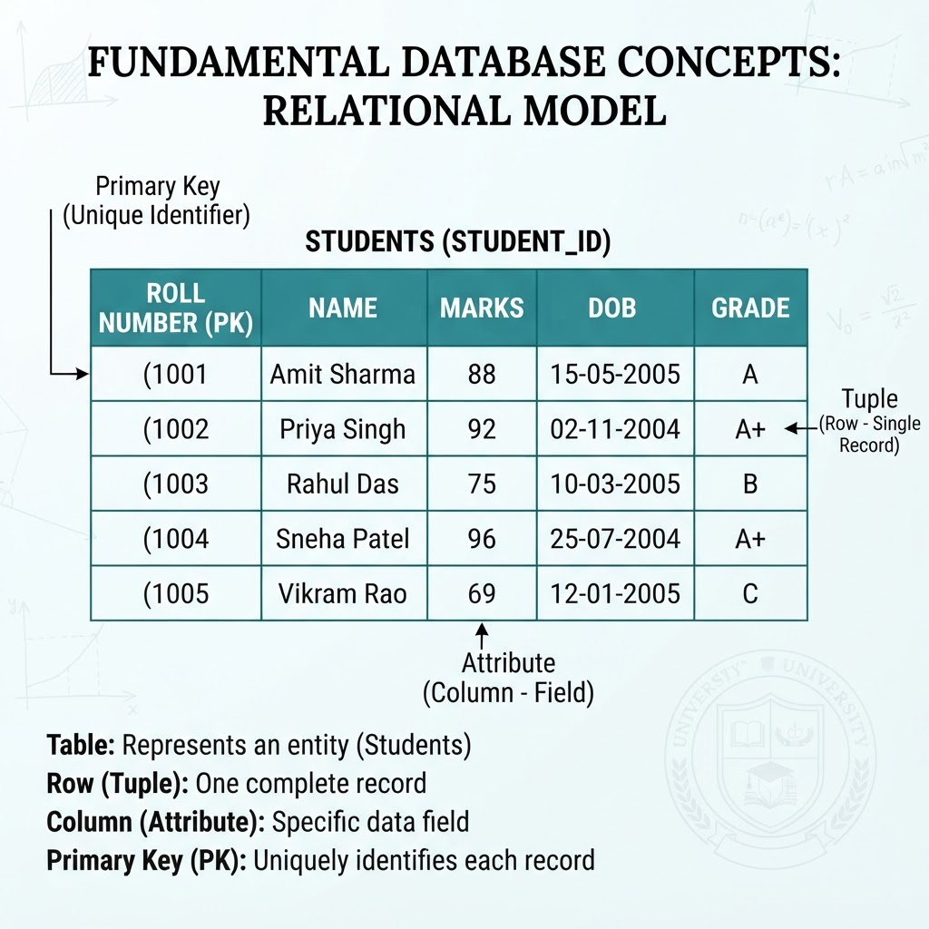
Components of Table:
Data Item (Field) or Attributes/Column:
A data item is the smallest unit of named data. It may consist of any number of bits or bytes. A data item represents one type of information and is often referred to as a field or data element.
Record/Row/Tuple:
A record is a named collection of data items which represents a complete unit of information.
Table/Relation:
A table is a named collection of all occurrences of a given type of logical record. A table is also called a relation in relational database.
10. Database Objects
- Table: It is a collection of data elements (values). It consists of vertical columns and horizontal rows where we put the required information.
- Columns or Fields or Attributes: It is a set of data values of a particularly simple type, one for each row of the table.
- Rows or Records or Tuples: It represents a single data item in a table. Every row in the table has the same structure.
11. Data Types
These are used to identify which type of data we are going to store in the database.
Integer Data Types:
| Data Type | Description | Range (Signed) | Storage Size |
|---|---|---|---|
| TINYINT | Very small integer | –128 to 127 | 1 byte |
| SMALLINT | Small integer | –32,768 to 32,767 | 2 bytes |
| MEDIUMINT | Medium-sized integer | –8,388,608 to 8,388,607 | 3 bytes |
| INT or INTEGER | Regular integer | –2,147,483,648 to 2,147,483,647 | 4 bytes |
| BIGINT | Large integer | –9,223,372,036,854,775,808 to 9,223,372,036,854,775,807 | 8 bytes |
Note: These can be UNSIGNED to store only positive values (range doubles on the positive side).
Decimal / Floating Point Types:
Used for real numbers (numbers with decimal points). Useful for storing money, measurements, etc.
| Data Type | Description | Syntax |
|---|---|---|
| FLOAT(M,D) | Approximate floating-point with precision | M = total digits, D = digits after decimal |
| DOUBLE(M,D) | Double-precision floating-point | Similar to FLOAT |
| DECIMAL(M,D) | Exact fixed-point number | M = total digits, D = digits after decimal |
Date and Time Types:
- DATE: YYYY-MM-DD format
- DATETIME: YYYY-MM-DD HH:MM:SS format
- TIMESTAMP: Similar to DATETIME format
- TIME: HH:MM:SS format
String/Text Data Types:
- CHAR: 1 to 255 characters (fixed length)
- VARCHAR: 1 to 65,535 characters (variable length)
- BLOB or TEXT: Up to 65,535 characters
BLOB (Binary Large Object):
BLOB stands for Binary Large Object. It is a data type in MySQL used to store binary data, such as images (JPEG, PNG), audio files (MP3), video files (MP4), and documents (PDF, DOCX).
| Data Type | Maximum Size | Usage |
|---|---|---|
| TINYBLOB | 255 bytes | Small binary files |
| BLOB | 65,535 bytes (~64 KB) | Medium-size files |
| MEDIUMBLOB | 16,777,215 bytes (~16 MB) | Larger files |
| LONGBLOB | 4,294,967,295 bytes (~4 GB) | Very large files |
12. MySQL and SQL
Processing Capability of SQL:
- Data Definition Language (DDL)
- Interactive Data Manipulation Language
- Embedded Data Manipulation Language
- View Definition
- Authorization
- Integrity
- Transaction Control
Data Dictionary:
A Data Dictionary is a file that contains "Metadata" (data about data).
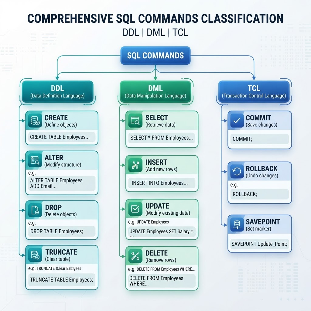
Classification of SQL Statements:
- Data Definition Language (DDL) Commands/Data Control Language
- Data Manipulation Language (DML) Commands
- Transaction Control Language (TCL) Commands
- Session Control Commands
- System Control Commands
13. DDL Commands
A data definition language (DDL) is a computer language used to create and modify the structure of database objects in a database.
Create, Alter and Drop Schema Objects:
Examples: CREATE TABLE, ALTER TABLE, DROP TABLE, CREATE INDEX, ALTER INDEX, DROP INDEX, RENAME TABLE, TRUNCATE
Grant and Revoke Privileges:
This section of DDL commands is used to grant or revoke permissions or privileges to work upon schema objects. For example, a user who creates a table becomes the owner of the table. The owner of the table can allow others to work on his/her table. This can be achieved by granting privilege for the same to others. This section is also known as Data Control Language (DCL) commands.
Maintenance Commands:
Examples: ANALYZE TABLE, CHECK TABLE, REPAIR TABLE, RESTORE TABLE
14. DML Commands
A Data Manipulation Language (DML) is a language that enables users to access or manipulate data as organized by the appropriate data model.
DML Operations:
- The Retrieval/SELECT of information stored in the database
- The Insertion of new information into the database
- The Deletion of information from the database
- The Modification of data stored in the database
Types of DML:
- Procedural DML: Requires a user to specify what data is needed and how to get it
- Non-procedural DML: Requires a user to specify what data is needed without specifying how to get it
Examples of DML Statements:
- To insert a tuple in a table: INSERT INTO statement is used
- To modify a tuple in a table: UPDATE statement is used
- To delete a tuple in a table: DELETE statement is used
- Other DML statements: SELECT, LOCK TABLE
15. TCL Commands
A transaction is one complete unit of work. To manage and control the transactions, the transaction control commands are used.
TCL Commands:
- COMMIT: Makes all the changes made by statements issued permanent
- ROLLBACK: Undoes all changes since the beginning of a transaction or since a savepoint
- SAVEPOINT: Makes a point up to which all earlier statements have been successfully completed
- SET TRANSACTION: Establishes properties for the current transaction
16. Database in MySQL
Creating Database:
Syntax:
CREATE DATABASE [IF NOT EXISTS] <database name>;
The IF NOT EXISTS clause tests whether a database already exists. If it does, the command is ignored; otherwise, a new database is created.
Opening Database:
USE <database name>;
Display Databases:
SHOW DATABASES;
Search Similar Database:
SHOW DATABASES LIKE '%student%';
Deleting Database:
DROP DATABASE <database name>;
17. Creating Tables
Tables are defined with the CREATE TABLE command. When a table is created, its columns are named and data type and size are supplied for each column. Each table must have at least one column.
Syntax:
CREATE TABLE <table name>(
  <column name> <datatype> <size>,
  <column name> <datatype> <size>,
  ...
);
Example:
CREATE TABLE class12(
  Roll_no INT(4),
  Name CHAR(20),
  mark INT(3),
  Mark DECIMAL
);
18. Data Integrity Through Constraints
A constraint is a condition or check applicable on a field or set of fields. There are two types: Column constraints (applicable to one column) and Table constraints (applicable to a group).
Different Constraints:
- Unique constraints
- Primary key constraints
- Default constraints
- Check constraints
- Foreign key constraints
Unique Constraint:
Ensures that no two rows have the same value in the specified column(s).
Primary Key Constraint:
Declares a column as the primary key of the table. The primary key cannot allow NULL values.
Default Constraint:
When a user does not enter a value for the column, the defined default value is automatically inserted in the field.
Check Constraint:
Limits values that can be inserted into a column of a table.
Foreign Key Constraint:
In an RDBMS, tables reference one another through common fields and to ensure validity of references, referential integrity is enforced.
19. Viewing and Inserting Data
Viewing a Table Structure:
DESC <tablename>;
OR
DESCRIBE <tablename>;
Viewing the List of Tables:
SHOW TABLES;
Inserting Data into Tables:
INSERT INTO <tablename> VALUES(value1, value2, value3...);
Multi-line Insertion:
INSERT INTO <tablename> (Col1, Col2, Col3)
VALUES (val1, val2, val3),
       (val1, val2, val3);
20. Making Simple SELECT Queries
The SELECT command in SQL lets you make queries on the database.
Syntax:
SELECT <column_name>, <column_name>
FROM <table_name>
WHERE <condition>;
Selecting All Columns:
SELECT *
FROM <tablename>;
Using DISTINCT Keyword:
The DISTINCT keyword eliminates duplicate rows from the results of a SELECT statement.
Using Column Aliases:
Columns selected in a query can be given a different name for output purposes.
SELECT Firstname AS "Name"
FROM <tablename>;
21. WHERE Clause - Selecting Specific Rows
The WHERE clause specifies the criteria for selection of rows to be returned in a SELECT statement. Only certain rows are needed from large tables.
Syntax:
SELECT <col_name>
FROM <tablename>
WHERE <condition>;
Relational Operators:
To compare two values, relational operators are used: = (equals), < (less than), > (greater than), <= (less than or equal), >= (greater than or equal), <> (not equal)
SELECT *
FROM <tablename>
WHERE <col_name> < 10;
Logical Operators:
- AND: True if all conditions are TRUE
- OR: True if any condition is TRUE
- NOT: True if condition is NOT TRUE
AND Example:
SELECT *
FROM <tablename>
WHERE col1 > 10 AND col2 > 15;
OR Example:
SELECT *
FROM <tablename>
WHERE col1 > 10 OR col2 > 15;
Combining AND, OR, and NOT:
SELECT *
FROM student
WHERE Roll_No > 103 AND (Mark < 70 OR Mark > 80);
22. Eliminating Redundant Data - DISTINCT Keyword
The DISTINCT keyword eliminates duplicate rows from the results of a SELECT statement.
Syntax:
SELECT DISTINCT <col_name>
FROM <tablename>;
ALL Keyword (Default):
If ALL is specified, the result retains duplicate rows. This is the default behavior.
SELECT ALL <col_name>
FROM <tablename>;
23. Condition Based on Range - BETWEEN and IN
BETWEEN Operator:
The BETWEEN operator defines a range of values that the column values must fall into. The range includes both lower and upper values.
SELECT <col>, <col>
FROM <tablename>
WHERE <ROLLNO> BETWEEN 100 AND 250;
NOT BETWEEN:
SELECT <col>, <col>
FROM <tablename>
WHERE <ROLLNO> NOT BETWEEN 100 AND 250;
IN Operator:
The IN operator selects values that match any values in a given list of values.
SELECT *
FROM <table_name>
WHERE <col_name> IN (val1, val2, val3, val4);
NOT IN:
SELECT *
FROM <table_name>
WHERE <col_name> NOT IN (val1, val2, val3, val4);
24. Condition Based on Pattern Matches - LIKE
SQL includes a string matching operator LIKE for comparisons on character strings using patterns. Patterns are case-sensitive.
Wildcard Characters:
- Percent (%): Matches any substring
- Underscore (_): Matches any single character
Pattern Examples:
- 'san%' matches any substring beginning with 'san'
- '%idge%' matches any string containing 'idge'
- '____' matches any string of exactly 4 characters
- '___%' matches any string of at least 3 characters
Syntax:
SELECT <col_name>, <col_name>
FROM <table_name>
WHERE <col_name> LIKE '13%';
25. Handling NULL Values
A field with NULL values is a field with no values. It is not possible to test for NULL values with comparison operators (=, <, >). Use IS NULL and IS NOT NULL instead.
IS NULL:
SELECT <col>, <col1>
FROM <tablename>
WHERE <col> IS NULL;
IS NOT NULL:
SELECT <col>, <col1>
FROM <tablename>
WHERE <col> IS NOT NULL;
IFNULL() Function:
Substitute NULL with a value in the output using IFNULL() function.
SELECT name, birth, IFNULL(CLASS, "12")
FROM <tablename>;
26. Sorting Results - ORDER BY Clause
The ORDER BY clause allows sorting of query results by one or more columns. The default order is ascending (ASC). Use DESC for descending order.
Ascending Order (Default):
SELECT <colname>
FROM <table name>
WHERE <Predicate>
ORDER BY <column name> ASC;

Example:
SELECT *
FROM student
ORDER BY Name;
Descending Order:
SELECT <colname>
FROM <table name>
WHERE <Predicate>
ORDER BY <column name> DESC;

Example:
SELECT *
FROM student
ORDER BY Mark DESC;
ORDER BY Multiple Columns:
SELECT *
FROM student
ORDER BY DOB DESC, Mark ASC;
27. Modifying Data - UPDATE Command
The UPDATE command modifies existing records in a table. The WHERE clause specifies which records to update. Use SET keyword for new data.
Syntax:
UPDATE <table name>
SET <column> = value
WHERE <condition>;
Update Multiple Columns:
UPDATE <table name>
SET <column1> = value1, <column2> = value2
WHERE <condition>;
Using Expressions in UPDATE:
UPDATE <table name>
SET Mark = Mark + 5
WHERE Roll_No > 100;
28. Deleting Data - DELETE Command
The DELETE statement removes rows from a table. The WHERE clause specifies which records to delete. DELETE removes entire rows, not individual field values.
Syntax:
DELETE FROM <table name>
WHERE <Predicate>;
Delete All Records:
DELETE FROM <table name>;
DROP TABLE Command:
Drop an entire table from the database.
DROP TABLE [IF EXISTS] <table name>;
29. ALTER TABLE Command
The ALTER TABLE command changes definitions of existing tables. It can add columns, delete columns, modify column definitions, or add constraints.
29.1 Adding a Column:
ALTER TABLE <table name>
ADD <col_name> <data type> <size> [FIRST|AFTER column];
29.2 Modify Column Definitions:
ALTER TABLE <table name>
MODIFY (column_name new_datatype(new size));
29.3 Changing a Column Name:
ALTER TABLE <tablename>
CHANGE [COLUMN] old_col_name new_col_name datatype size;

Example:
ALTER TABLE <tablename>
CHANGE First_name FirstName VARCHAR(20);
29.4 Add Constraint:
ALTER TABLE table_name
ADD CONSTRAINT constraint_name PRIMARY KEY (column_name);

Example:
ALTER TABLE employees
ADD CONSTRAINT pk_emp_id PRIMARY KEY (emp_id);
29.5 Drop Column:
ALTER TABLE <table name>
DROP COLUMN <col_name>;
29.6 Rename Table:
ALTER TABLE <table name>
RENAME TO <new_table name>;
30. Detailed Constraints - Syntax and Examples
30.1 NOT NULL Constraint:
Ensures a column cannot have NULL values.
CREATE TABLE Student (
  Roll_No INT NOT NULL,
  Name VARCHAR(50) NOT NULL,
  Email VARCHAR(100)
);
30.2 UNIQUE Constraint:
Ensures all values in a column are unique. Multiple UNIQUE constraints can exist.
CREATE TABLE Student (
  Roll_No INT PRIMARY KEY,
  Email VARCHAR(100) UNIQUE
);
30.3 PRIMARY KEY Constraint:
Uniquely identifies each row. Cannot be NULL. Only one PRIMARY KEY per table.
CREATE TABLE Student (
  Roll_No INT PRIMARY KEY,
  Name VARCHAR(50),
  Mark INT
);

OR using table constraint:
CREATE TABLE Student (
  Roll_No INT,
  Name VARCHAR(50),
  Mark INT,
  PRIMARY KEY (Roll_No)
);
30.4 DEFAULT Constraint:
Sets a default value for a column when no value is inserted.
CREATE TABLE Student (
  Roll_No INT PRIMARY KEY,
  Name VARCHAR(50),
  Class VARCHAR(10) DEFAULT "12"
);
30.5 CHECK Constraint:
Limits the values that can be inserted into a column.
CREATE TABLE Student (
  Roll_No INT PRIMARY KEY,
  Name VARCHAR(50),
  Mark INT CHECK (Mark >= 0 AND Mark <= 100)
);
30.6 FOREIGN KEY Constraint:
References the primary key of another table. Maintains referential integrity.
CREATE TABLE Faculty (
  emp_id INT PRIMARY KEY,
  name VARCHAR(100),
  F_ID INT,
  FOREIGN KEY (F_ID) REFERENCES Courses(F_ID)
);
30.7 ON DELETE CASCADE and ON UPDATE CASCADE:
ON DELETE CASCADE: Automatically deletes child records when parent record is deleted.
ON UPDATE CASCADE: Automatically updates child records when parent foreign key is updated.
ALTER TABLE faculty
ADD CONSTRAINT fk_faculty_id
FOREIGN KEY (F_ID) REFERENCES courses(F_ID)
ON UPDATE CASCADE
ON DELETE CASCADE;
30.8 ALTER Constraint Examples:
-- Add PRIMARY KEY:
ALTER TABLE employees
ADD CONSTRAINT pk_emp_id PRIMARY KEY (emp_id);

-- Drop CONSTRAINT:
ALTER TABLE employees
DROP CONSTRAINT pk_emp_id;

-- Modify DEFAULT:
ALTER TABLE Student
ALTER Class SET DEFAULT "12";
31. GROUP BY Clause
The GROUP BY clause combines records that have identical values in particular fields. Creates one summary record per group when used with aggregate functions.
Syntax:
SELECT column, COUNT(*)
FROM table_name
GROUP BY column;
Example - Count by Department:
SELECT job, COUNT(*)
FROM employee
GROUP BY job;
GROUP BY Multiple Columns:
SELECT deptno, COUNT(empno)
FROM employee
GROUP BY deptno;
32. Joins
A join combines rows from two or more tables based on a related column between them. Joins are used to retrieve related data from multiple tables.
32.1 Cartesian Product (Cross Join):
A Cartesian product combines every row of the first table with every row of the second table. If table A has 3 rows and table B has 4 rows, result will have 3 × 4 = 12 rows.
Syntax:
SELECT *
FROM table1, table2;
Example:
SELECT *
FROM Student, Course;
32.2 Equi-Join (Inner Join):
An Equi-join combines rows from two tables when they have matching values in a specified column. The WHERE clause specifies the join condition using equality (=) operator.
Syntax:
SELECT <col1>, <col2>, ...
FROM <table1>, <table2>
WHERE <table1>.<common_col> = <table2>.<common_col>;
Example:
SELECT Student.Roll_No, Student.Name, Course.Course_Name
FROM Student, Course
WHERE Student.Course_ID = Course.Course_ID;
32.3 Natural Join:
A Natural Join combines tables based on columns that have the same name and data type. No WHERE condition is needed. Duplicate columns appear only once.
Syntax:
SELECT *
FROM <table1>
NATURAL JOIN <table2>;
Example:
SELECT *
FROM Student
NATURAL JOIN Course;
32.4 Table Aliases:
Use short names for tables to make queries shorter and more readable. Aliases are temporary alternate names for tables.
Syntax:
SELECT <alias1>.<col>, <alias2>.<col>
FROM <table1> <alias1>, <table2> <alias2>
WHERE <alias1>.<col> = <alias2>.<col>;
Example:
SELECT s.Roll_No, s.Name, c.Course_Name
FROM Student s, Course c
WHERE s.Course_ID = c.Course_ID;
33. Aggregate Functions
Aggregate functions perform calculations on a set of rows and return a single result. They are often used with GROUP BY clause to group results.
33.1 COUNT() Function:
Returns the number of rows matching the specified criteria.
Syntax:
SELECT COUNT(*)
FROM <table_name>;

SELECT COUNT(column_name)
FROM <table_name>;
Examples:
-- Count all rows
SELECT COUNT(*) FROM Student;

-- Count non-NULL values in a column
SELECT COUNT(Email) FROM Student;

-- Count with condition
SELECT COUNT(*) FROM Student WHERE Mark > 70;
33.2 SUM() Function:
Returns the sum of all values in a numeric column. Ignores NULL values.
Syntax:
SELECT SUM(column_name)
FROM <table_name>;
Examples:
-- Sum all marks
SELECT SUM(Mark) FROM Student;

-- Sum with condition
SELECT SUM(Mark) FROM Student WHERE Class = '12';

-- Sum with alias
SELECT SUM(Mark) AS Total_Marks FROM Student;
33.3 AVG() Function:
Returns the average of values in a numeric column. Ignores NULL values and divides by the count of non-NULL values.
Syntax:
SELECT AVG(column_name)
FROM <table_name>;
Examples:
-- Average of all marks
SELECT AVG(Mark) FROM Student;

-- Average with condition
SELECT AVG(Mark) FROM Student WHERE Roll_No > 100;

-- Average with rounding
SELECT ROUND(AVG(Mark), 2) FROM Student;
33.4 MAX() Function:
Returns the maximum value from a column. Works with numeric, character, and date data types.
Syntax:
SELECT MAX(column_name)
FROM <table_name>;
Examples:
-- Maximum mark
SELECT MAX(Mark) FROM Student;

-- Maximum mark with alias
SELECT MAX(Mark) AS Highest_Mark FROM Student;

-- Maximum with WHERE clause
SELECT MAX(Mark) FROM Student WHERE Class = '12';
33.5 MIN() Function:
Returns the minimum value from a column. Works with numeric, character, and date data types.
Syntax:
SELECT MIN(column_name)
FROM <table_name>;
Examples:
-- Minimum mark
SELECT MIN(Mark) FROM Student;

-- Minimum mark with alias
SELECT MIN(Mark) AS Lowest_Mark FROM Student;

-- Minimum with WHERE clause
SELECT MIN(Mark) FROM Student WHERE Roll_No > 105;
33.6 Aggregate Functions with GROUP BY:
Combine aggregate functions with GROUP BY to calculate results for different groups.
Examples:
-- Average mark per class
SELECT Class, AVG(Mark)
FROM Student
GROUP BY Class;

-- Maximum mark per class
SELECT Class, MAX(Mark)
FROM Student
GROUP BY Class;

-- Count students per class
SELECT Class, COUNT(*)
FROM Student
GROUP BY Class;

-- Sum marks per department
SELECT Dept, SUM(Mark)
FROM Student
GROUP BY Dept;
33.7 HAVING Clause with Aggregates:
HAVING clause filters groups created by GROUP BY based on aggregate function results. Use WHERE for filtering rows before grouping, and HAVING for filtering groups after aggregation.
Syntax:
SELECT column, COUNT(*)
FROM table_name
GROUP BY column
HAVING COUNT(*) > value;
Examples:
-- Classes with more than 30 students
SELECT Class, COUNT(*)
FROM Student
GROUP BY Class
HAVING COUNT(*) > 30;

-- Departments with average marks greater than 70
SELECT Dept, AVG(Mark)
FROM Student
GROUP BY Dept
HAVING AVG(Mark) > 70;